Green Tea and Velociraptors

“If you want to inspire confidence, give plenty of statistics. It does not matter that they should be accurate, or even intelligible, as long as there is enough of them.” Lewis Carroll (1832-1898)

 

The last post on this series gave an introduction to the background and significance of quantitative shape analysis. I conveyed the use of landmarks, or geometric co-ordinates, as the basis for statistical analysis of shape. The last article finished by stating this article would discuss different methods of geometric morphometric analysis, but I forgot one crucial step: Data Collection! Here, I present a simple and efficient way of collecting data for use as the basis for a range of geometric morphometric analyses.

Following is an example of data collection from a simple coursework study I did last year, looking at cranial allometry in carnivores. Firstly, you need a target or hypothesis for your analysis. The target here was to use exemplar carnivorous mammal species to look at shape variation in the skull, and to interpret in terms of form and dietary function. The first decision to make is what points to use as your landmark data. I’ll use a hypothetical skull as an example.

 

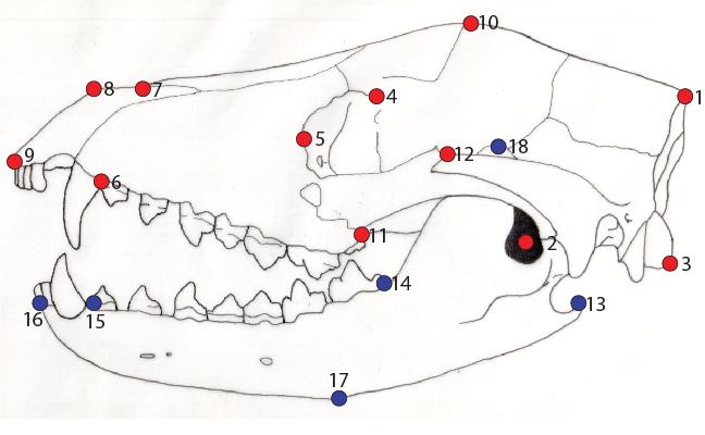
Each one of these landmarks represents a specific topographically correspondent point amongst all specimens in the sample. For the sake of simplicity in this example, assume that the lower jaw and the cranium are a single module. The landmarks can be defined as such:

Cranial landmarks (right-lateral aspect; red)

1. Posterior extremity of occipital margin (type 3)

2. Tympanic aperture (centre) (type 1)

3. Posteroventral extremity of occipital condyle (type 3)

4. Ventral extremity of dorsal postorbital process (type 3)

5. Rostral extremity of orbital periphery (type 3)

6. Mid-point on ventral maxillary margin between premolars and canines (type 3)

7. Ventral deflection in dorsal margin (maximum curvature) [rostral to postorbital] (type 2)

8. Dorsal expansion in dorsal margin (maximum curvature) [posterior to external nares] (type 2)

9. Anterior extremity of premaxilla (type 3)

10. Dorsal extremity of dorsal margin (type 3)

11. Ventral extremity of zygamatic arch-jugal suture (type 1)

12. Position of distal border on posterior-most tooth (maxillary) (type 1)

 

Lower jaw landmarks (right-lateral aspect; blue)

13. Posterior extremity of angular process (type 3)

14. Posterior-most (distal) extent of dentary molars (type 3)

15. Mid-point on ventral dentary margin between premolars and canines (type 3)

16. Anterior extremity of dentary (type 3)

17. Point of posterodorsal deflection of ventral margin, culminating in angular process (type 2)

18. Ventral pinnacle of coronoid process (dentary) (type 2)

 

This is just a hypothetical example to show landmark positions and how to define them. Real data is freely available for almost anything on the internet. A series of sample images can be easily obtained through MorphBank, for example. If anyone reading this would like, I can send them a copy of the images I used for this coursework as a trial data set – just drop me a quick message with your email address.

Converting these landmarks into usable geometric data is possible through a number of image modification programs. A good one to use is ImageJ, freely available on the web. An important thing to note at this point is that within your image collection, every one you import into this program or any other must be angularly identical, or as close as possible (e.g., all of a precise lateral view of a skull).

Using ImageJ you can simply import an image with pre-defined landmarks as above, use the ‘Point’ tool to click on the landmark, hit ctrl-m (or use the Analyse-Measure tab), and hey-presto, you have the two-dimensional geometric co-ordinate of that point in a table! Consecutive points can then be added to this table for each specimen. Do this for all points per sample in a pre-defined numerical sequence (as indicated above), then simply export to an Excel spread-sheet. A rather nifty thing you can then do is plot them as a graph, and you’ll see a landmark representation of your image (awesomeness of this depends on how many landmarks you use). Repeat for all samples, and you have a comparable data set. Simple eh! Note that this can be done free of scale, so you don’t need to measure any lengths or inter-landmark distances. A future post will cover how to compensate for this in quantitative shape analysis. What you want to end up with at this stage is a single spread-sheet, with a labelled tab for each specimen, and containing a series of geometric co-ordinates that are topographically related between specimens.

There are of course more techniques using more complex software and data imaging methods (using surface or outline data, laser scans etc.), but typically these will not be accessible to the general public. The above procedure is a convenient and free method of obtaining a decent and workable initial data set, without having to spend endless time in a museum collection or laboratory.

So, now you know the procedure, nothing should stop anyone from going out there and collecting a data set, constructing a series of landmarks and digitally obtaining their geometric co-ordinates. Right? Next time, I’ll actually discuss how to assemble this data into a format that you can use to input to some free software, and several analyses you can then conduct with this software (e.g., Principal Components Analysis).